Lab 8: Spectral Reflectance

Goals and Objectives

Within this lab, spectral reflectance from satellite images were measured and interpreted. Spectral signatures were collected from a provided image, then later graphed. Analysis was performed on the verified their spectral separability within the signature mean plots.

Methods

To begin the lab, the provided image was opened within Erdas. To collect spectral signatures, the Drawing tab was clicked, followed by the Polygon function. Once this was activated, a polygon is drawn around the desired surface type. From here the Raster tab is clicked. Next, the Supervised button is clicked and the Signature Editor is selected. Now, the Signature Editor is opened. Within the window, a new signature is added by clicking the Create New Signature form AOI button. Once the signature row appears, the Signature Name and color is able to be changed.

The collection of the standing water polygon, with its spectral curve

Next the Signature Mean Plot can be observed by pressing the Display Mean Plot Window button. The background color of the graph can be edited by selecting Edit, followed by Chart Options. Here a lighter color can be selected within the dropdown box. For this lab, the first surface type analyzed was Standing Water. The Signature Mean Plot looks as followed.

Signature mean plot of standing water

Throughout the rest of the lab, eleven other surface types were analyzed. All signature mean plots were gathered through the same processed previously used, however they were gathered within the same Signature Editor window.  The eleven other signature plots appeared as followed.

Signature mean plot of moving water

Signature mean plot of vegetation

Signature mean plot of riparian vegetation

Signature mean plot of crops

Signature mean plot of urban grass

Signature mean plot of dry soil

Signature mean plot of moist soil

Signature mean plot of rock

Signature mean plot of asphalt highway

Signature mean plot of airport runway

Signature mean plot of concrete surface (parking lot)

After all of these spectral signatures were collected, the Switch Between Single and Multiple Signature Mode was clicked within on of the Spectral Mean Plot windows. This allows you to observe all spectral signatures at once. Here, you can analyze similarities between the objects reflectance. The table below indicates which band wavelength had the highest and lowest reflectance for all surfaces.

Signature	Material/Surface	Highest (µm)	Lowest (µm)
1	Standing water	0.45	0.63 and 10.40
2	Moving water	0.45	10.40
3	Vegetation	0.77	10.40
4	Riparian vegetation	0.77	0.63 and 10.40
5	Crops	0.77	0.63 and 10.40
6	Urban grass	0.77	0.63 and 10.40
7	Dry soil	1.55	0.63
8	Moist soil	0.45	10.40
9	Rock	0.45	10.40
10	Asphalt highway	1.55	0.77
11	Airport runway	0.63 and 1.55	0.77
12	Concrete surface (Parking lot)	0.45	0.77

Results

The spectral curves of all twelve surfaces collected

Lab 7: Stereoscopy and Orthorectification

Goals and Background:
In this lab, photogrammetric skills were practiced using aerial and satellite images to become familiarized with calculations used to determine the scale, feature measures, and relief displacement. Other processes such as stereoscopy and orthorectification were introduced in this lab as well.


Methods:

Part 1: Scales, measurements and relief displacement

Section 1: Calculating scale of nearby vertical aerial photographs

First the scale of a photograph was found by using a ruled and finding the distance in inches between the two marked points marked on the photograph. Next, this number was divided by the real life distance once it was converted into inches. For example, the scale of this photograph was 1:38,498.

S=PD/GD
PD: Photograph distance
GD: Real world distance 

2.75 in/8822.47 feet *12

2.75 in/ 105869.64 = 1/38,498

Next, the scale of another image was found with a different method using the focal length of the camera. The cameras focal length was divided by the value of the altitude above sea level subtracted by elevation of the land. For example, the scale of this photograph was 0.0079.

S= f/ H- h
S= Scale
f= focal length
H= altitude above sea level
h= elevation

152mm/ (20,000ft – 796ft) = 0.0079

Section 2: Measurements of area of features on aerial photographs

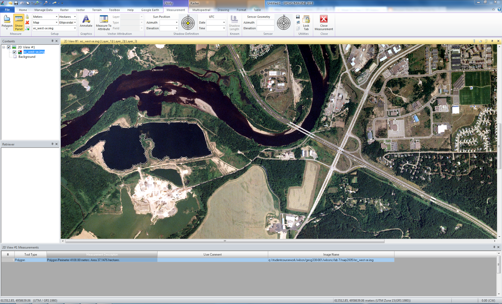
Using the polygon tool under the Method button on the Erdas tool bar, the area and perimeter of th lagoon within the following image was found. By clicking on the Polyline, followed by the Polygon function, the tool can be activated. Next points were laid around the perimeter of the lagoon. After double clicking once the end is reached, the value was generated in the panel and the bottom of the screen. The units could be adjusted using the drop down box on the upper tool bar.

Section 3: Calculating relief displacement from object height

Here, the relief displacement for an objects height was determined. First, real world height was multiplied by the divided by the radial distance of the feature from the principle point.  Next, the

d= h *r/H
d= relief displacement

h= height of object (real world)

r= radial distance of the top of the displaced object from the principle point

H= height of camera above the local datum

(0.375in * 3209)*(10.5in)/3980ft =

1203*375ft *10.5/47760 = 0.26in  

In relation to the principle point, because the relief displacement value is positive the feature must be plotted inwards.

Part 2: Stereoscopy

Here, the method used generates a 3-dimensioanl perspective of the city of Eau Claire. First, two separate images were opened into separate viewers within Erdas. Next under the Terrain tab, the Anaglyph function was selected. Here the window appeared and each photo was selected as an input. The output location and name was determined, and exaggeration was changed to 2.00. The following image was generated.

Part 3: Orthorectification

In this part of the lab, Erdas Image Lecia Photogrammetric Suite (LPS) was used to orthorectify images to create planimetrically accurate orthoimages.

Section 1: Create Project

First, in Erdas, the Toolbox tab was selected, followed by the LPS function. In this window, the New Block File was selected. Under the Geometric Model Category and choose Polynomial-base Pushbroom. Under this SPOT Pushbroom was selected. After okay was selected, another window appears. Under the Horizontal Reference Coordinate System, the Set button was clicked. This opens the Projection Chooser window. Within this window, several changes were made to fit the directions parameters. Okay was selected.

Section 2: Add imagery to the Block and define sensor model

Next, an image was added by highlighting the image folder, then selecting the Add Frame button. The desired image was then added. Next, the Show and Edit Frame Properties icon was selected to open the next function. Within this next window, the edit button was selected and all parameter was accepted. This changed the Int. column to now appear green.

Section 3: Activate Point measurement tool and collect GCPs

Here the Start point measurement tool was activated. A window appeared, where the settings were changed to "classic point measurement tool". Next, this opens the full Point measurement window. Before GCPs were added, the GCP Reference Source dialog box popped up, and the Image layer option was chosen. This activated the Reference Image Layer window, where the desired image was then added. Now in the present window, the User Viewer as Reference checkbox is selected to add the reference image to the left portion of the window.

To begin adding GCP's to the reference image. Once the desired area of the GCP was found, the Add button was selected, followed by the Create Point button. This was then placed in the desired XY coordinate position. Following this, the corresponding point was added to the Block image, on the right on the window. This was completed by selecting the Create Point button, and once again selecting the desired area. This process was repeated 2 more time until the Automatic (x,y) Drive button was selected to approximate the position of the GCP block file. After this, 6 more GCP's were added to the images.

Next, the data was saved. From here, 2 other GCP's were added but the Point # was changed. First the Reset Horizontal Reference Source was selected. In the window that pops up, the Image Layer option was selected. Now, a new window appears and the desire image is selected. After Okay is selected, the new image is added to the left side of the viewer. To make a distinction between the previous GCP's, the next Point # is changed from 10 and 11, to 11 and 12. Now these are saved and the Use Viewer As Reference box is deselected.

The next set is to select the Reset Vertical Reference Source button. This opens a new window called Vertical Reference Source. Here all parameters given within the directions were selected. Once this is closed, the all rows were selected and the Update Z values on Selected Points was selected to update the Z values of the selected reference points. These are then deselected.

Section 4: Set Type and Usage, add a 2nd image to the block and collect its GCP's

This next process begins with highlighting the column Type, and right-clicking to select the Formula option. Within the textbox, Full was written. Apply is selected, and the process is repeated with Usage column, however Control is typed into the textbox. Save is selected again.

Now, point collection of the reference image is finished and the block image needs to have points added. The Add Frame button is selected, and the desired block image is added. The row corresponding to the image was selected, followed by the Frame Properties function where all default parameters were accepted. From here the Point measurement button was selected, followed by the Classic Point Measurement tool. From here GCP's were collected in the same manner as before.

Once the desired area is found in the left image, the Create Point button was selected, and the GCP was placed. The X and Y file of this point will now appear in the bottom right window. Now, from the previous points collected, only points located within this new image are collect. Here, the final GCP's were added and the points were saved.

Section 5: Automatic tie point collection, triangulation and ortho resample

Here, the Automatic Tie Point Generation Properties button is selected and the parameters according to the directions were chosen in all tabs. The function was then Run.

From here, Edit was selected to find the Triangulation Properties function. This was opened, and the desired values were selected, followed by running the function. This is followed by the Triangulation Summary Report window. Clicking Report with open up the Summary dialog box that can be saved. From here, Accept is clicked, and the Ext. column has now turned green.

Triangulation Summary Report

Now, the Start Ortho Resampling button was selected. The designated parameters and output images were selected. Here, Bilinear Interpolation was selected, and a single output was added in the bottom window of the dialog box. Here, a second window pops up and the Input file and location are verified. This process is repeated to add a second single output. Now, Okay was selected to run the Ortho Resampling process.

Section 6: Viewing the orthorectified images

Now, next to the Orthos folder on the left side of the view, the + button is selected. One image is highlighted then right-clicked on to select the View function. This is brought into Erdas. The second image is opened into the same Erdas viewer. The swipe function was used to observe the accuracy of the special overlap.

Results

Image orthospot_pan.img on left, and orthospot_panb on left: Swipe function applied

Image orthospot_pan.img on left, and orthospot_panb on left: Swipe function applied

Lab 6: Geometric Correction

Goals and Background
In this lab, image processing was practiced through the use of geometric correction. Two type of two types of geometric correction was used, called Image-to-Map Rectification, and Image-to-Image Registration.

Methods

Part 1: Image-to-Map Rectification

First, under the Multispectral tab, Control Points was selected. From there, Polynomial was selected within the window.

From here, the Multipoint Geometric Correction window popped up, and all default settings were accepted. Next, the reference image was selected. After this the Reference Map window pops up, and okay was selected. Following this, the Polynomial Model Properties window appears and all default settings are accepted once Close is selected.  

Now, in the Multipoint Geometric Correction window, all points into the lowest box were deleted. After both the reference image and imput image were "fit to screen", new GCP points were added. Specifically, 4 points were added to both images. After specific adjustments were completed by zooming , the RMS error and the Total RMS Error were less than 2.0.

Part 2: Image to image registration

Two images were opened in the different viewers. One had significant image distortion. Again, the Multispectral tab was selected, following the Control Points button. For the following windows, the default settings were accepted. In the Polynomial Model Properties box, the polynomial order was changed to 3. From here, 12 GCP's were added simultaneously to the input image and the reference image.

After all points had an RMS error less than 1, and the Total RMS error was less than 1, the Display Resample Image Dialog button was selected. Here, the output image was named, and the settings in the Method box were changed to Bilinear Interpolation. From here, Okay was selected and the output image was generated.

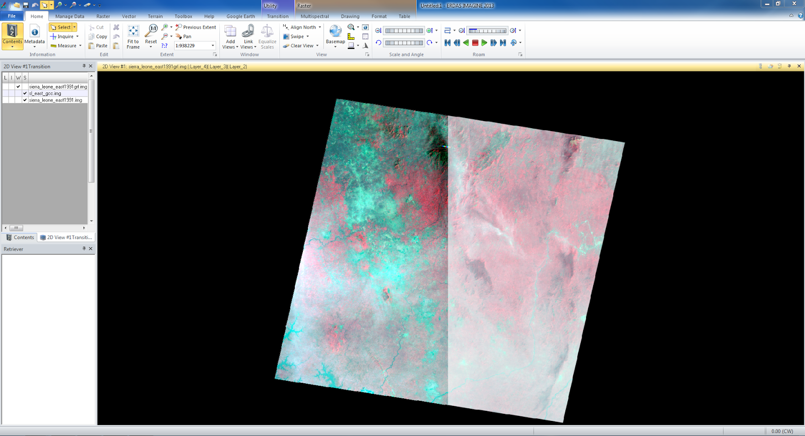
Next, the output image was overlapped on the reference image. The distortion between the images appears to be almost inexistent. This appears below.

The reference image appears on the left, and the output image appears on the right.

    

Lab 5: Image Mosaic, Image Enhancement, Band Ratio, and Binary Change

Goals and Background
This lab covers different analytical processes that are typically used within real life remote sensing projects. The tools such as image mosaic, spatial and spectral image enhancement, band ratio, and binary change detection were practiced in this lab.

Methods

Part 1: Image mosaicking

Image mosaicking is necessary when the specific area you are interested is expands throughout more than one image. It is necessary to mosaic these images together to create a seemless image of the specific area. Two types of mosaicking were practiced in this lab. First, two adjacent satellite images were opened in Erdas one the same layer. These are opened separately. Before uploading the first selected image, the Multiple tab was selected to choose the Multiple Images in Virtual Mosaic. Next, the Raster tab was selected to specify first that the background transparent option is selected, and second that the fit to frame option is selected. The image was then opened. The same steps for both the Multiple and Raster tabs were completed for the second image. Once they are both opened, the images will be slightly overlapped.

Section 1: Image mosaic with the us of Mosaic Express

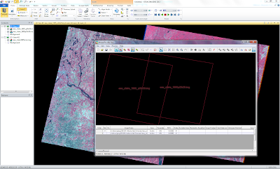
Once the images are overlapped, the Raster tab was selected. The Mosaic button was selected, followed by the Mosaic Express function. This opens the Mosaic Express window as shown

.

Within this window, the folder button was selected to open up the desired image. The images are selected in the order, that which ever is selected first will lay on top of the image that is selected second. From here, the final tab labeled Output was selected. Next the folder button was clicked to designate where the output image would be saved, and also to name the output image. The following image includes the original photos on the left, and the output images on the right.

Section 2: Image mosaic with the use of MosaicPro

Next, Mosaic Pro was used to generate an output image that will appear more blended, with the separate image edges being harder to discern. First, the previously generated output images were opened however the same functions under the Multiple and Raster tab as before. Now, the Mosaic tab was again selected under Raster, however this time the MosaicPro function was used. The MosaicPro window was then activated. The Add Images button was then selected to open another window. Now the desired image was selected. Following this, the Image Area Options tab was selected where the Commute Active Area function was chosen. After this, clicking Okay finalized this step. These steps are then completed for the following image.

The generated output image looked as follows.

From here, the Color Corrections button was selected on the tool bar to open up it's dialog box. Here, the Use Histogram Mating button was then selected and next the Set button was clicked, which opened up the Histogram Matching window. In the first drop down box, Overlap Areas was selected. From here, Okay was selected on both windows to complete this stage. These windows appeared as follows.

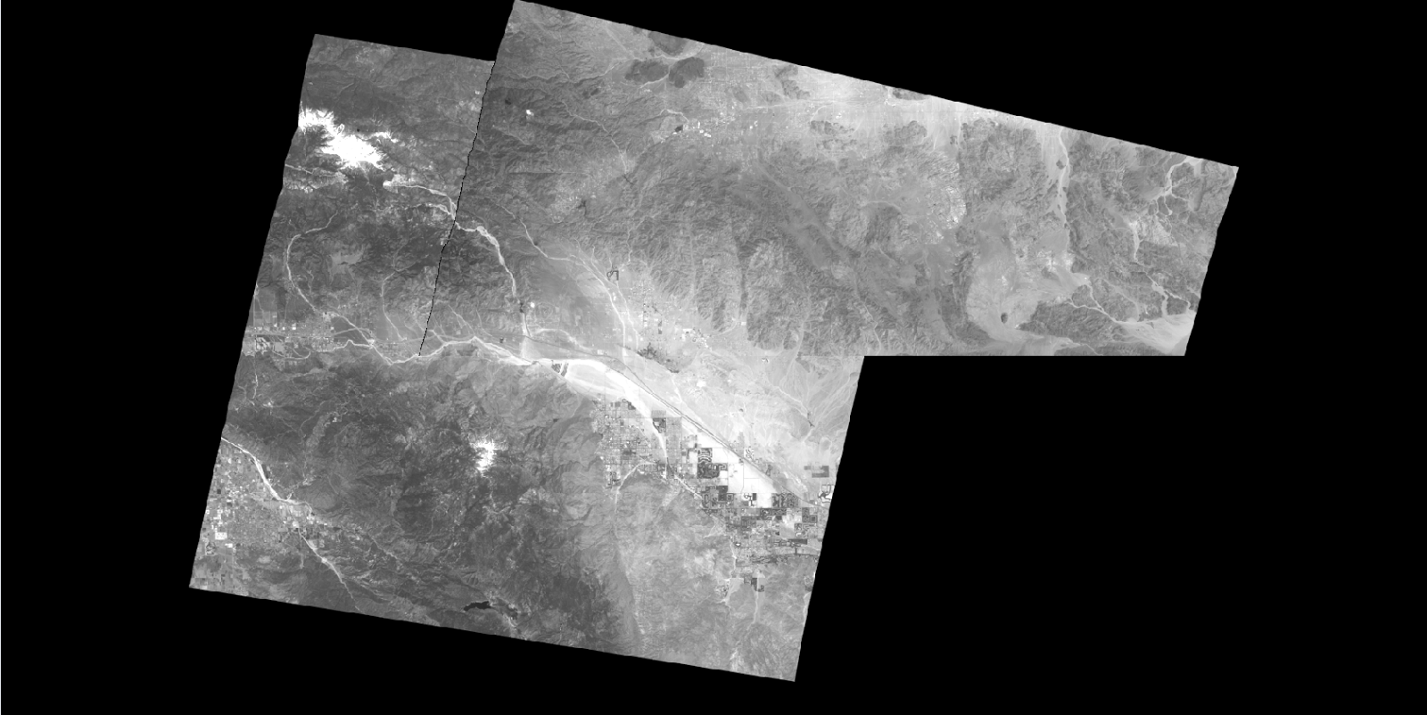
Back to working in the MosaicPro window, the Process function was selected, followed by the Run Mosaic button. Next, the desired folder for the output image was selected. Here, the desired image output name was created as well. After clicking Okay, the following output image was generated.

Part 2: Band Ratioing

Band ratioing was completed in this part of the lab by using the  NDVI,  normalized difference vegetation index. In Erdas, the desired image was opened. The Raster tab was the selected, followed by the Unsupervised button, then the NDVI function. The Indices window appeared. Here, the current image was selected for the input file, and the desired image output name and folder location were selected for the output. The sensor Landsat 4 TM - 6 bands was selected. Under function, NDVI was chosen.

From here, Okay was selected, and the output image was generated and the outcome looks as followed.

Part 3: Spatial and spectral Image enhancement

Section 1: Spatial enhancement

In this section of the lab, spatial enhancement techniques were used. First, the desired image was opened in Erdas. From here, the Raster tab was selected. Next, the Spatial button was clicked, followed by the Convolution function. The Convolution window appeared and 5x5 Low Pass was selected under Kernal type. The desired imput image was then selected, followed by naming the output image and selecting the desired folder location.

The Ouput image that was generated is to the right of the following photo, while the original photo is to the left.

Next, with another image, the same process was completed through the Convolution function. However, for this photo 5x5 High Pass under kernel was selected. After the input and output setting have been completed as before, and the new image was generated by clicking Okay.

The Ouput image that was generated is to the right of the following photo, while the original photo is to the left.

Edge Enhancement: Using edge enhancement, the edges were enhanced to makes them more distinguishable within the image. First, a new image was opened into Erdas. Again the Convolution function was use again as above. However, 3x3 Laplacian Edge Detection was selected under Kernel. In addition, the Fill box under Handle Edges by was checked, and the Normalize the Kernel button was unchecked. Again, the input and output option were specified, and Okay was clicked to generate the output.

The Ouput image that was generated is the following photo.

Section 2: Spectral enhancement

Here, two linear contrast stretches were completed to increase the visible quality of the image. To begin, an image was brought into Erdas. By clicking the Metadata icon at the top right of the tool bar, the histogram of the image is found in the Histogram tab. Here, there was only one mode present. This allowed a minimum-maximum stretch to be completed. To run this, the Panchromatic tab was selected. From here, the General Contrast icon was selected, followed by the General Contrast function. This opens up the Contrast Adjust window. Here, in the Method window, Gaussian is selected.

After Apply was clicked, the following image was generated.

Next, another image was opened in Erdas. The histogram for this image was observed again, which consisted of several modes, mean this image had a non-Gaussian histogram. Due to this, a Piecewise stretch is used for this image. This was done so by under entering the General Contrast options, however this type Piecewise Contrast was selected. From here, the Contrast Tool window was opened. By placing the curser over the histogram, the range of each mode was determined. These values were entered into the respective "low", "middle", and "high" boxes. The last value in the "high" box was then extended to 180.

After Apply was clicked, the following Piecewise image was generated.

Histogram Equalization: This function was used to improve the contrast of the image in order to facilitate visual interpretation. To begin this process, an image was opened into Erdas. Again, the histogram was observed and found to have one mode. To increase the limited contrast in this photo, a histogram equalization was used. First, the Raster tab was opened, and the Radiometric button was clicked. From here, the Histogram Equalization function was selected which opened up it's window.

Next, the input image was designated and OK was selected.

Part 4: Binary change detection (image differencing)

Here, this function was used to find where the pixels differed between the two years, which is found through a generated difference image. First, the two desired photos to compare were opened in separate viewers. The Raster tab was selected, followed by the Functions option. From there, Two Image Functions was selected to open up the Two Input Operator's window. Here, the older image was entered into the input file, where the other older image was entered into input #2. The output file was then given a name and put into the desired folder. Within this window, the Layer option under both input #1 and #2 was changed to layer 4. After clicking okay the generated output looked as follows.

Section 1: Histogram observations

To determine the change seen, observations needed to be completed by calculation. The Metadata of this image was used, such as the Standard Deviation and the Mean, as well as the center X coordinate of the histogram. Two values of change-no change were calculated by:

1) Std. Dev x 1.5= Total + Mean = Total + Middle X coordinate= Upper Point
2) Middle X Coordinate  - (Std. Dev x 1.5= Total + Mean = Total) = Lower Point

This two values were then added to the image's histogram.

Section 2: Mapping change pixels in difference image using spatial modeler

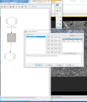
With this method, negative values will be removed from the difference image that was generated previously, to overall easily show the changes that occurred between the two selected images. To begin, and the Toolbox tab is selected. From here, Model Marker was clicked, followed by the Model Marker function. This opens a window called New Model. Here, two Raster objects were added, connected by a Function, which was then connected to an additional Raster object. The result looked as shown below.

By double clicking on each item, the desired photo was able to be input in the top two Raster Objects. From there, an equation was inserted into the Function object once again by double clicking on the image. The equation should consist of: The Oldest Image - The Earlier Image + the given constant. After this, the last Raster object was double clicked on to design an output name for the difference image, and a file location for it.

Now, this image is opened up into a view on Erdas. The same routine in Model Maker to develop a model for another output image. One Raster object is connected to one Function object, is then connected to one final Raster object. The difference image is selected to be the input for the first Raster object. In the Function object, the Function drop down box was changed to Conditional, and below this EITHER/IF was selected. An equation was entered into the lowest box, which included the photo name > the determined threshold value.

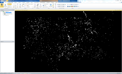
After this is all entered, the last Raster object was selected. Here the final difference output name and location was selected. The Run was run and the final output image looked as shown below.

Lastly, this image was brought into ArcMap. Here the colors of Change and No changed where designed, and the background color was removed. Furthermore, a legend, scale, and North Star symbol were added. The final generated map is shown below.

Results:

Final Outputs from the lab

Part 1: MosaicExpress

MosaicPro

Part 2: NDVI Output:

Part 3: Lowpass Output

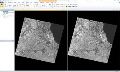
The right image is the Lowpass output

Highpass Output:

 

Laplacian Output:

The right image is the Laplacian Output

Minimum-Maximum Stretch Output:



Piecewise Output:

Histogram Equalization:

 Part 4: Model Maker

Final Eau Claire County Map Output: